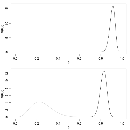
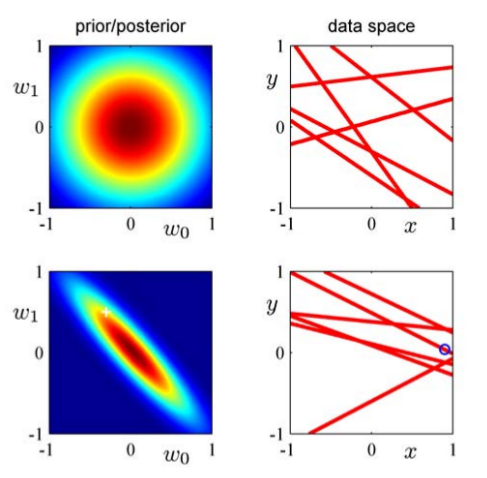
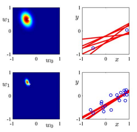
class: center, middle, inverse, title-slide # Introduction ## Curso JAE ICMAT 2021 ### Roi Naveiro ### 2021-06-24 --- <script type="text/x-mathjax-config"> MathJax.Hub.Config({ TeX: { Macros: { Xcal: "{\\mathcal{X}}", Xbf: "{\\mathbf{X}}", Zbf: "{\\mathbf{Z}}", Vbf: "{\\mathbf{V}}", Hbf: "{\\mathbf{H}}", Rbb: "{\\mathbb{R}}" }, extensions: ["AMSmath.js","AMSsymbols.js"] } }); </script> # Outline 1. Intro, basic concepts: belief and probability, exchangeability. Conjugate models. 2. MC approximation, MCMC methods: Gibbs, Metropolis, Hamiltonian Montecarlo. 3. Scalable inference: variational Bayes and Stochastic Gradiente Langevin Dynamics. 3. AI applications. --- # Slides and Labs * [Github](https://github.com/roinaveiro/curso-Bayes-JAE) * **Disclaimer**: This session's material comes from Ch. 1,2 and 3 of Hoff's book. Hoff, P. D. (2009). A first course in Bayesian statistical methods (Vol. 580). New York: Springer. --- # Probability and Bayesian inference * Informally: a way to express our degree of certainty about unknown things. * Formally: a numerical way of representing rational beliefs. * There is a relation between probability and information. * Bayes' rule is a rational method for updating beliefs given new information. --- # Bayesian learning (on a nutshell) * Statistical induction: Learn about population given sample. * Learn about `\(\theta\)` given dataset `\(y\)`. * After observing dataset, we have less uncertainty about `\(\theta\)` than before. Bayes **quantifies** this change. * Notation: sample space `\(\mathcal{Y}\)`; parameter space `\(\Theta\)`. --- # Bayesian learning (on a nutshell) * The process: 1. Set a *prior* `\(p(\theta)\)` describing our belief that `\(\theta\)` represents the truth. 2. Set a *sampling model* `\(p(y \vert \theta)\)` that describes our belief that `\(y\)` would be the outcome of our study if `\(\theta\)` wa true. 3. Compute *posterior* `\(p(\theta \vert y)\)`, that describes our belief that `\(\theta\)` is the truth after having observed `\(y\)`. $$ p(\theta \vert y) = \frac{p(y \vert \theta) p(\theta)}{\int_{\Theta} p(y \vert \tilde{\theta}) p(\tilde{\theta}) d \tilde{\theta}} $$ * Mathematical justification in Savage(1954, 1972). --- # Beliefs * Say, `\(Be(F)\)`, represents **numerically** our beliefs about a statement. * Can be formalized using bets ( `\(Be(F) > Be(G)\)` means we would prefer to bet `\(F\)` is true than `\(G\)` is true). * Axioms of beliefs: 1. `\(Be(\text{not } H | H ) \leq Be(F | H ) \leq Be( H | H )\)` 2. `\(Be( F \text{or } G | H ) \geq \max \lbrace Be(F | H ), Be(G | H ) \rbrace\)` 3. `\(Be( F \text{and } G | H ) \text{ can be derived from } Be(G | H ) \text{ and } Be(F | G \text{ and } H)\rbrace\)` * Probability satisfies this axioms. --- # Exchangeability * Let `\(p(y_1, \dots, y_n)\)` be the joint density for `\(Y_1, \dots, Y_n\)`. If `\(p(y_1, \dots, y_n) = p(y_{\pi_1}, \dots, y_{\pi_n})\)` for all permutations `\(\pi\)` then `\(Y_1, \dots, Y_n\)` are exchangeable. * If `\(\theta \sim p(\theta)\)` and `\(Y_1, \dots, Y_n\)` are conditionally i.i.d. given `\(\theta\)`, then marginally `\(Y_1, \dots, Y_n\)` are exchangeable. (Prove it). * The other way around? De Finetti's theorem. --- # De Finetti's theorem Suppose that `\(\lbrace Y_1, Y_2, \dots \rbrace\)` is a potentially infinite sequence of random variables with common sampling space. If for any `\(n\)` `\(Y_1, \dots, Y_n\)` is exchangeable, then $$ p(y_1, \dots, y_n) = \int \left \lbrace \Pi_1^n p(y_i \vert \theta) \right \rbrace p(\theta) d \theta $$ for some parameter `\(\theta\)`, some prior and sampling model, that depend on our belief model `\(p(y_1, \dots, y_n)\)`. --- # Why Bayes? * Provides a natural and principled way of combining prior information with data, within a solid decision theoretical framework * It provides inferences that are conditional on the data and are exact, without reliance on asymptotic approximation. * Bayesian analysis also can estimate any functions of parameters directly. * Likelihood principle. * It provides interpretable answers, such as “the true parameter has a probability of 0.95 of falling in a 95% credible interval. * UQ in a fundamental way! --- # Why not Bayes? * Computational cost. --- class: middle, center, inverse # One-parameter models --- # The binomial model * A sample of 129 people (from a population of `\(N\)`) are asked whether or not they are happy. `\(Y_i=1\)` if happy `\(Y_i=0\)` if not. * `\(\theta = \sum_{i=1}^N Y_{i} / N\)`. * `\(p(y_1, \dots, y_n \vert \theta) = \theta^{\sum_{i=1}^{129} y_i} (1-\theta)^{129 -\sum_{i=1}^{129} y_i}\)` * Prior? --- # Uniform prior * `\(p(\theta) = 1\)` for all `\(\theta \in [0,1]\)`. * Posterior? Using Bayes rule: `\begin{equation*} p(\theta \vert y_1, \dots, y_{129}) = \frac{p(y_1, \dots, y_{129} \vert \theta ) p(\theta)}{p(y_1, \dots, y_n)} \end{equation*}` `\begin{equation*} p(\theta \vert y_1, \dots, y_{129}) \propto \theta^{118} (1-\theta)^{11} \end{equation*}` * Normalizing constant? Identify with kernel of beta with parameters `\(a=119\)` and `\(b=12\)`. `\begin{equation*} \frac{x^{a-1}(1-x)^{b-1}} {B(a,b)}\! \end{equation*}` * Proof --- # Uniform and beta prior * Same result for every sequence with the same number of 1s. * `\(y = \sum_{i} y_i\)` is a sufficient statistic. -- * `\(p(y | \theta) = \binom{n}{y} \theta^y (1-\theta)^{n-y}\)` * Posterior: `\(p(\theta | y) = \text{beta}(y+1, n-y+1)\)` . * Uniform is a particular case of beta (with parameters 1, 1). What if we choose a general beta prior? `\begin{equation*} p(\theta | y ) \propto p(\theta)p(y | \theta) = \theta^{a+y-1} (1-\theta)^{b+n-y-1} \end{equation*}` * So `\(p(\theta | y) = beta(a+y, b + n -y)\)` --- # Conjugacy * A class `\(\mathcal{P}\)` of prior distributions for `\(\theta\)` is called cojugate for a sampling model `\(p(y | \theta)\)` if `\begin{equation*} p(\theta) \in \mathcal{P} \Rightarrow p(\theta \vert y) \in \mathcal{P} \end{equation*}` Make life easier... but we loose flexibility. * Note that `\begin{eqnarray*} \text{E}[\theta | y] = \frac{a+y}{a+b+n} = \end{eqnarray*}` `\begin{eqnarray*} \frac{a+b}{a+b+n} \times \text{prior expectation} + \frac{n}{a+b+n} \times \text{data avg.} \end{eqnarray*}` Take a look at the asymptotic behaviour... --- # The example <!-- --> --- --- # Prediction * Say we want to predict a new observation. * Bayesian data analysis does it in a formal way `\begin{equation*} \text{Pr}(\tilde{Y} = 1 \vert y_1, \dots, y_n) = \int \text{Pr}(\tilde{Y} = 1 \vert \theta, y_1, \dots, y_n) p(\theta \vert y_1, \dots, y_n) d \theta \end{equation*}` `\begin{equation*} = \int \theta p(\theta \vert y_1, \dots, y_n ) d \theta = \frac{a+ \sum_{i=1}^n y_i}{a+b+n} \end{equation*}` --- # Confidence regions * We can ask the posterior **any question**... * ... like which are the regions of the parameter space that are likely to contain the true value of the parameter. * **Bayesian coverage** An interval `\([l(y), u(y)]\)` has `\(95 \%\)` of Bayesian coverage for `\(\theta\)` if `\begin{equation*} \text{Pr}(l(y) < \theta < u(y)) | Y=y) = 0.95 \end{equation*}` * **Highest posterior density region**: a `\(100 \times (1-\alpha) \%\)` HDP region consist of a subset `\(s(y)\)` of the parameter space such that 1. The probability that the true value lies within the region is `\(1-\alpha\)` 2. If `\(\theta_a \in s(y)\)`, and `\(\theta_b \notin s(y)\)` then `\(p(\theta_a | Y=y) > p(\theta_b | Y=y)\)` --- # Example  --- # The Poisson model * Say `\(\mathcal{Y} = \lbrace 0, 1, 2, \dots \rbrace\)` * If we model `\(Y_1, \dots, Y_n\)` as conditional iid samples from a Poisson of mean `\(\theta\)` `\begin{equation*} \text{Pr} (Y_1=y_1, \dots, Y_n=y_n \vert \theta) \prod_{i=1}^n \frac{1}{y_i !} \theta^{y_i} e^{-n \theta} \propto \theta^{\sum y_i} e^{-n \theta} \end{equation*}` * `\(\sum_{i=1}^n Y_i\)` is sufficient, and `\(\sum_{i=1}^n Y_i \vert \theta \sim \text{Poisson}(n\theta)\)`. * What is the form of the conjugate prior? --- # Conjugate prior * Gamma distribution `\(p(\theta) = \frac{b^a}{\Gamma(a)} \theta^{a-1} e^{-b \theta}\)`. * Posterior is a `\(\text{gamma} (a + \sum_{i=1}^n Y_i, b+n)\)` (proof). `\begin{equation*} \text{E}[\theta \vert y_1, \dots, y_n] = \frac{b}{b+n}\frac{a}{b} + \frac{n}{b+n} \frac{\sum_i y_i}{n} \end{equation*}` * Predictive (proof): `\begin{equation*} p(\tilde{y} \vert y_1, \dots, y_n) = \int p(\tilde{y} \vert \theta) p(\theta \vert y_1, \dots, y_n) d \theta \end{equation*}` * Easy to solve... the predictive is a negative binomial. `\begin{equation*} \text{E}[\tilde{Y} \vert y_1, \dots, y_n] = \frac{a+ \sum_i y_i}{b+n} \end{equation*}` `\begin{equation*} \text{Var}[\tilde{Y} \vert y_1, \dots, y_n] = \text{E}[\theta \vert y_1, \dots, y_n]\times \frac{b+n+1}{b+n} \end{equation*}` * Lab --- # The normal model * If our sampling model is normal with mean `\(\theta\)` and variance `\(\sigma^2\)` `\begin{equation*} p(y_1, \dots, y_n \vert \theta, \sigma^2) \propto \exp \left \lbrace -\frac{1}{2} \sum \left( \frac{y_i - \theta}{\sigma}\right)^2 \right \rbrace \end{equation*}` * Assume we know the variance. Conjugate prior on `\(\theta\)` is normal `\((\mu_0, \tau_0^2)\)`. * Posterior is normal (proof) `\begin{equation*} \mu_n = \frac{\tilde{\tau}_0^2}{\tilde{\tau}_0^2 + n \tilde{\sigma}^2} \mu_0 +\frac{n \tilde{\sigma}^2}{\tilde{\tau}_0^2 + n \tilde{\sigma}^2}\bar{y} \end{equation*}` `\begin{equation*} \tilde{\tau}_n^2 = \tilde{\tau}_0^2 + n \tilde{\sigma}^2 \end{equation*}` * The predictive is a normal `\((\mu_n, \tau_n^2 + \sigma^2)\)` --- class: middle, center, inverse # More than one parameter models --- # The multivariate normal model * If our sampling model is multivariate normal with mean `\(\boldsymbol{\theta}\)` and covariance `\(\Sigma\)` `\begin{equation*} p(\boldsymbol{y}_1, \dots, \boldsymbol{y}_n \vert \boldsymbol{\theta}, \Sigma) \propto \exp \left \lbrace -\frac{1}{2} \sum_{i=1}^n (\boldsymbol{y}_i - \boldsymbol{\theta}^T ) \Sigma^{-1} (\boldsymbol{y}_i - \boldsymbol{\theta})\right \rbrace \end{equation*}` * With known covariance, assuming a multivariate normal `\((\boldsymbol{\mu}_0, \Lambda_0)\)` prior for `\(\boldsymbol{\theta}\)`... * The posterior is multivariate normal `\((\boldsymbol{\mu}_n, \Lambda_n)\)` `\begin{equation*} \Lambda_n = (\Lambda_0^{-1} + n \Sigma^{-1})^{-1} \end{equation*}` `\begin{equation*} \boldsymbol{\mu}_n = (\Lambda_0^{-1} + n \Sigma^{-1})^{-1} (\Lambda_0^{-1} \boldsymbol{\mu}_0 + n \Sigma^{-1} \bar{\boldsymbol{y}}) \end{equation*}` --- # Regression * We observe pairs `\((y_i, \boldsymbol{x}_i)\)`. * We want to describe how the sampling distribution of `\(y\)` varies with `\(x\)`. * The sampling model is `\begin{equation*} \epsilon_1, \dots, \epsilon_n \sim \mathcal{N}(0, \sigma^2) \end{equation*}` `\begin{equation*} Y_i = \boldsymbol{\beta}^T \boldsymbol{x}_i + \epsilon_i \end{equation*}` * Then `\begin{equation*} p(y_1, \dots, y_n | \boldsymbol{x}_1, \dots, \boldsymbol{x}_n, \boldsymbol{\beta}, \sigma^2) \propto \exp \left \lbrace - \frac{1}{2 \sigma^2} \sum_{i=1}^n (y_i - \boldsymbol{\beta}^T \boldsymbol{x}_i)^2 \right \rbrace \end{equation*}` * Or `\begin{equation*} \boldsymbol{y} \vert \boldsymbol{X}, \boldsymbol{\beta}, \sigma^2 \sim \mathcal{N} (\boldsymbol{X} \boldsymbol{\beta}, \sigma^2 \boldsymbol{I}) \end{equation*}` --- # Regression * If: `\(\boldsymbol{\beta} \sim \mathcal{N} (\boldsymbol{\beta}_0, \Sigma_0)\)`, then the posterior is a multivariate density `\begin{equation*} \text{Var}[\boldsymbol{\beta} | \boldsymbol{y}, \boldsymbol{X}, \sigma^2] = (\Sigma_0^{-1} + \boldsymbol{X}^T \boldsymbol{X} / \sigma^2)^{-1} \end{equation*}` `\begin{equation*} \text{E}[\boldsymbol{\beta} | \boldsymbol{y}, \boldsymbol{X}, \sigma^2] = (\Sigma_0^{-1} + \boldsymbol{X}^T \boldsymbol{X} / \sigma^2)^{-1} (\Sigma_0^{-1} \boldsymbol{\beta}_0 + \boldsymbol{X}^T \boldsymbol{y}/ \sigma^2 ) \end{equation*}` * If elements of `\(\Sigma_0^{-1}\)` are very small, the expectation is approx `\((\boldsymbol{X}\boldsymbol{X}^T)^{-1}\boldsymbol{X}^t \boldsymbol{y}\)`! * If `\(\sigma^2\)` is very large, the expectation is `\(\boldsymbol{\beta}_0\)`. * Exercise: proof that, if prior mean is zero, and covariance `\(\lambda \boldsymbol{I}\)`, the MAP of `\(\beta\)` is the solution of *ridge regression*. ---  ---  --- # Univariate Normal with unknown variance * We do inference in both, mean `\(\theta\)` and variance `\(\sigma^2\)`. * Conjugate prior: `\begin{eqnarray*} p(\theta, \sigma^2) = p(\theta | \sigma^2)p(\sigma^2) = \text{normal}(\mu_0, \tau_0 = \sigma/\sqrt{\kappa_0}) p(\sigma^2) \end{eqnarray*}` * For the variance `\begin{eqnarray*} 1/ \sigma^2 \sim \text{gamma}(\nu_0/2, \nu_0 \sigma_0^2/2) \end{eqnarray*}` * The posterior `\begin{eqnarray*} p(\theta, \sigma^2 | y_1, \dots, y_n) = p(\theta | \sigma^2, y_1, \dots, y_n)p(\sigma^2 | y_1, \dots, y_n) \end{eqnarray*}` --- # Univariate Normal with unknown variance * Mean  * Precision   --- # Univariate Normal with unknown variance * Super easy to sample from posterior!! * If `\(\tau_0\)` is not proportional to gamma... `\begin{equation*} \theta \sim \text{normal} (\mu_0, \tau_0^2) \end{equation*}` `\begin{equation*} 1/ \sigma^2 \sim \text{gamma}(\nu_0/2, \nu_0 \sigma_0^2/2) \end{equation*}` * The marginal posterior density of `\(1/\sigma^2\)` is not a gamma distribution, or any other dist. we can sample from easily. --- # Another intractable * Bayesian mixture model (blackboard).