ML for Molecular Properties Prediction
Simón Rodríguez Santana (ICMAT)
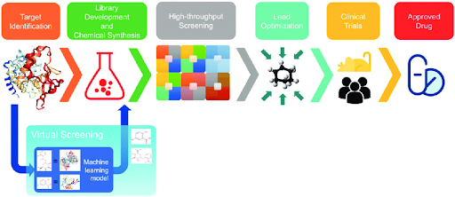
Discovering new molecules - Process
Design of new molecule: countless applications in various sectors, e.g. pharmaceuticals and materials.
Pharma: average time discovery starts - market, 13 years. Outside pharma: 25 years
![]()
Discovering new molecules - Process
![]()
The old and soon-to-be-old ways
Problems with previous approaches
Just existing molecules are explored
Much time lost evaluating bad leads
Goal: traverse chemical space more “effectively”: reach optimal molecules with less evaluations than brute-force screening
Mathematically speaking
Combinatorial optimization problem
Often stochastic and multi-objective
Black-box objective functions
Black-box constraints
De novo design
The process of automatically proposing novel chemical structures that optimally satisfy desired properties
![]()
This workshop
Session 1: Predictive (QSAR) Models, with focus in low data regime
Session 2: Generative Models
Session 3: The Tailor’s Drawer (+ Case Study)
Predictive Models
Predictive models to forecast properties of molecules given structure, with focus on small data regime
Computational representations of molecules
An overview of predictive models for molecular properties
Evaluating model performance
Representating molecules
Molecules are 3D QM objects with: nuclei with defined positions surrounded by electrons described by complex wave-functions
Digital encoding that serves as input to model
Uniqueness and invertibility
Trade-off: information lost vs complexity
1D, 2D and 3D Representations
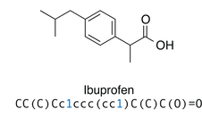
1D Representations
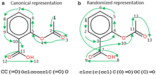
Simplified Molecular Input Line Entry System (SMILES)
Molecule as graph (bond length and conformational info lost)
Traverse graph
Generate Sequence of ASCII characters
![]()
2D Representations
- Nodes represent atoms
- Edges represent bonds
- Nodes/Edges have associated features (atom number, bond type, etc.)
- Capture connectivity!
- Respect symmetries
- Tailored algorithms (GNNs!)
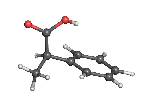
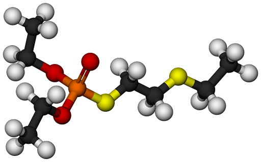
3D Representations
3D point clouds: \(\mathcal{M} = \lbrace x_i, r_i \rbrace_{i=1}^p\), where \(x_i\) are features and \(r_i\) are coordinates
Minimal information lost (conformational preferences, bond lengths, etc.)
Tailored predictive algorithms that respect 3D translational and rotational invariance
![]()
An overview of predictive models for molecular properties
Molecular representation \(x\) and property \(y \in \mathbb{R}\)
Given training data \(\mathcal{D} = \lbrace x_i, y_i \rbrace_{i=1}^p\)…
… predictive regression model of \(y\) given \(x\).
Deterministic models - Point Forecasts
Probabilistic (Bayesian) models - Probabilistic Forecasts
Models for 1D representations - Descriptors
Models for 1D representations - Strings
One-hot encoding of SMILES representations
Deep Neural Nets: RNN, 1D Conv, Transformers
BNNs
Models for 2D molecular representations
GNNs (on a nutshell)
Functions on graph-structured data
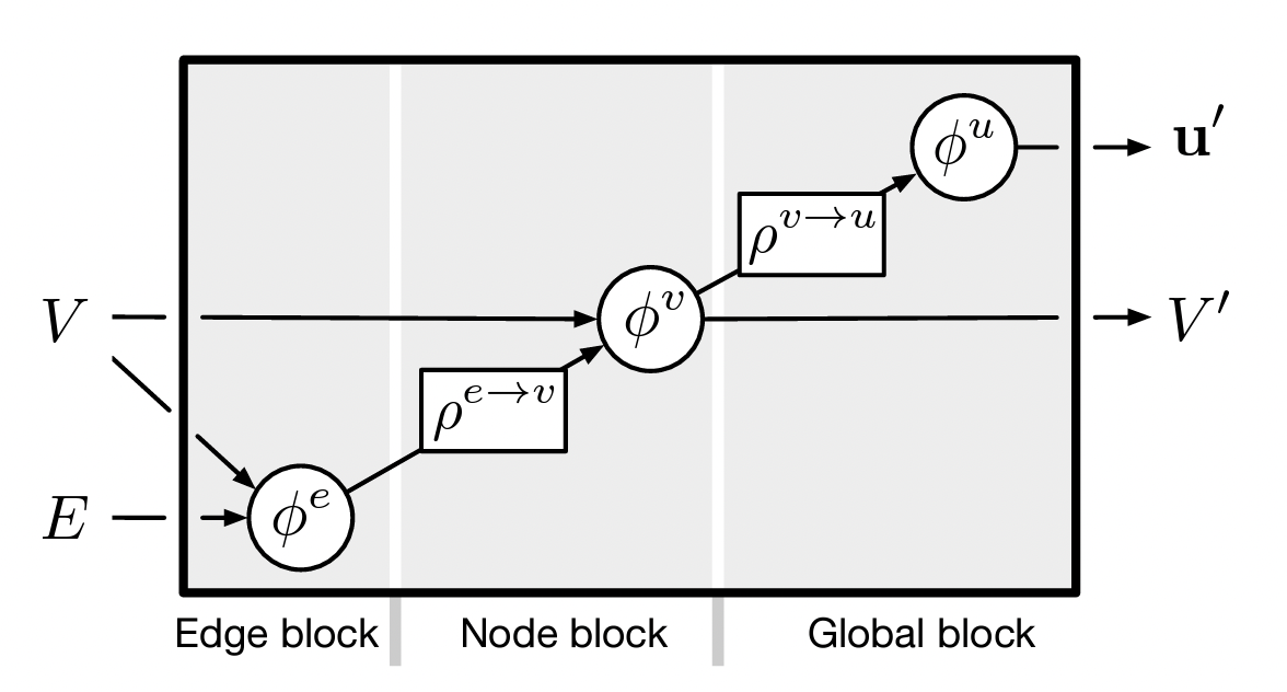
GN block (graph-to-graph map): primary computational unit in GNN
Graph \(N_v\) nodes and \(N_e\) edges: tuple \(G = (\textbf{u}, V, E)\)
- \(\textbf{u}\): global attribute
- \(V = \lbrace v_i \rbrace_{i=1:N^v}\): set of node attribute vectors
- \(E = \lbrace (\textbf{e}_k, r_k, s_k)\rbrace_{k=1:N^e}\): set of edges. \(\textbf{e}_k\) edge attribute, \(r_k\) index of receiving node, and \(s_k\) is index of sending node.
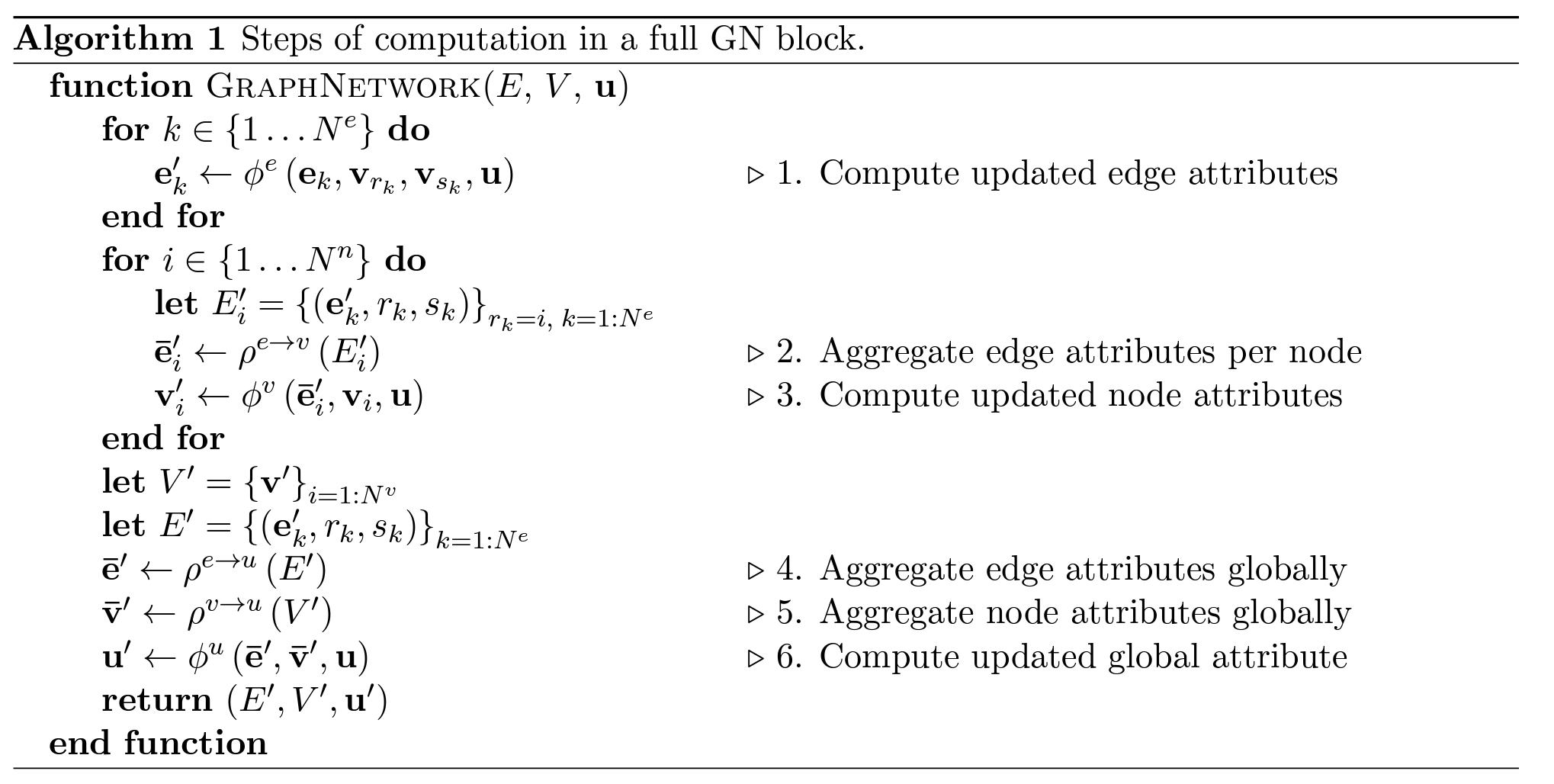
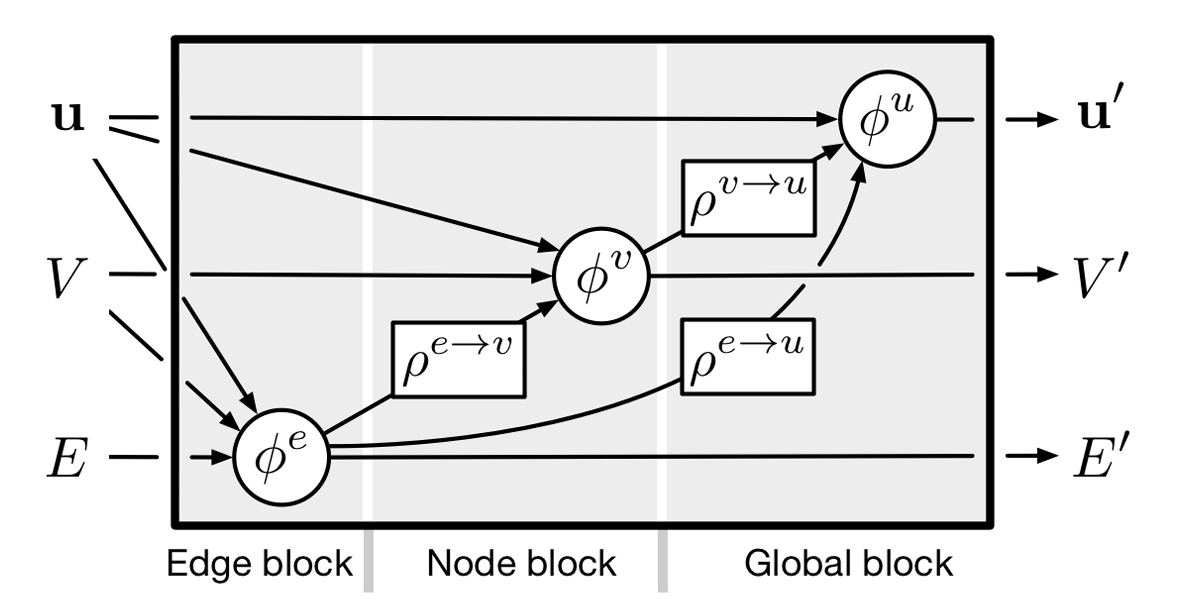
GN Block
Edge update function \(\phi^e\)
Node update function \(\phi^v\)
Global update function \(\phi^u\).
\(\rho^{e\rightarrow v}\): aggregates edge attributes per node
\(\rho^{e\rightarrow u}\): aggregates edge attributes globally
\(\rho^{v\rightarrow u}\): aggregates node attributes globally.
GN Block - Computations
![]()
GN Block - Computations
![]()
MPNN Block - Computations
![]()
GNN
Various parametric forms for functions
Multilayer perceptrons for the update functions and sums for the aggregate functions
GN blocks can be concatenated
Output layer of GNN depends on the task
GNN Workflow
The entire architecture can be summarized as follows:
Encode the input graph using independent node and edge update functions to match the internal node and edge feature sizes
Apply multiple GN blocks
Use an output layer to map the updated global features to a property prediction
Once the architecture is defined, the parameters can be optimized using standard optimizers and loss functions.
Models for 3D molecular representations
Geometric Neural Networks
(Again) many architectures
In a Geometric Net Block we update:
Node features, s.t. updated features are invariant to 3D translations and rotations
Node coordinates, s.t. updated coordinates are equivariant to 3D translations and rotations
\(E(n)\) equivariant graph neural nets Satorras et. al. (2022)
In a MPNN
\(\forall\) edges \(k\), \(\textbf{e}'_k = \phi^{e} (\textbf{e}_k, \textbf{v}_{r_k}, \textbf{v}_{s_k})\)
\(\forall\) nodes \(i\)
- \(E'_i = \lbrace (\textbf{e}'_k, r_k, s_k) \rbrace_{r_k = i}\)
- \(\bf{\overline{e}'_i} = \rho^{e\rightarrow v} (E'_i)\)
- \(\textbf{v}'_i = \phi^{v} (\bf{\overline{e}'_i}, \textbf{v}_{i})\)
- \(V' = \lbrace \textbf{v}'_i \rbrace_{i=1:N^v}\)
- \(\bf{\overline{v}}' = \rho^{v\rightarrow u} (V')\)
- \(\textbf{u}' = \phi^u (\bf{\overline{v}'})\).
E(n) equivariante GNNs
\(\forall\) edges \(k\), \(\textbf{e}'_k = \phi^{e} (\textbf{e}_k, \textbf{v}_{r_k}, \textbf{v}_{s_k}, \color{red}{\Vert x_{r_k} - x_{s_k} \Vert ^2} )\)
\(\forall\) nodes \(i\)
- \(E'_i = \lbrace (\textbf{e}'_k, r_k, s_k) \rbrace_{r_k = i}\)
- \(\bf{\overline{e}'_i} = \rho^{e\rightarrow v} (E'_i)\)
- \(\textbf{v}'_i = \phi^{v} (\bf{\overline{e}'_i}, \textbf{v}_{i})\)
- \(\color{red}{x'_i = x_i + C \sum_{k;~r_k = i} (x_i - x_{s_k}) \cdot \phi^x (\textbf{e}'_k)}\)
- \(V' = \lbrace \textbf{v}'_i \rbrace_{i=1:N^v}\)
- \(\bf{\overline{v}}' = \rho^{v\rightarrow u} (V')\)
- \(\textbf{u}' = \phi^u (\bf{\overline{v}}')\).
Evaluating quality of probabilistic predictions
Evaluating quality of probabilistic predictions
Idea: create \((100 \cdot q)\)% prediction intervals for the property prediction of every molecules in a test set.
\(C(q)\) is the proportion of the molecules in the test set whose property value is in the interval calculated for such molecule.
If \(C(q) = q\) we say that the model is well calibrated.
If \(C(q) < q\) we say that the model is overconfident.
If \(C(q) > q\) we say that the model is underconfident.
Evaluating quality of probabilistic predictions
![]()
Hands-on!
![]()