De-novo Molecular Design
De-novo molecular design
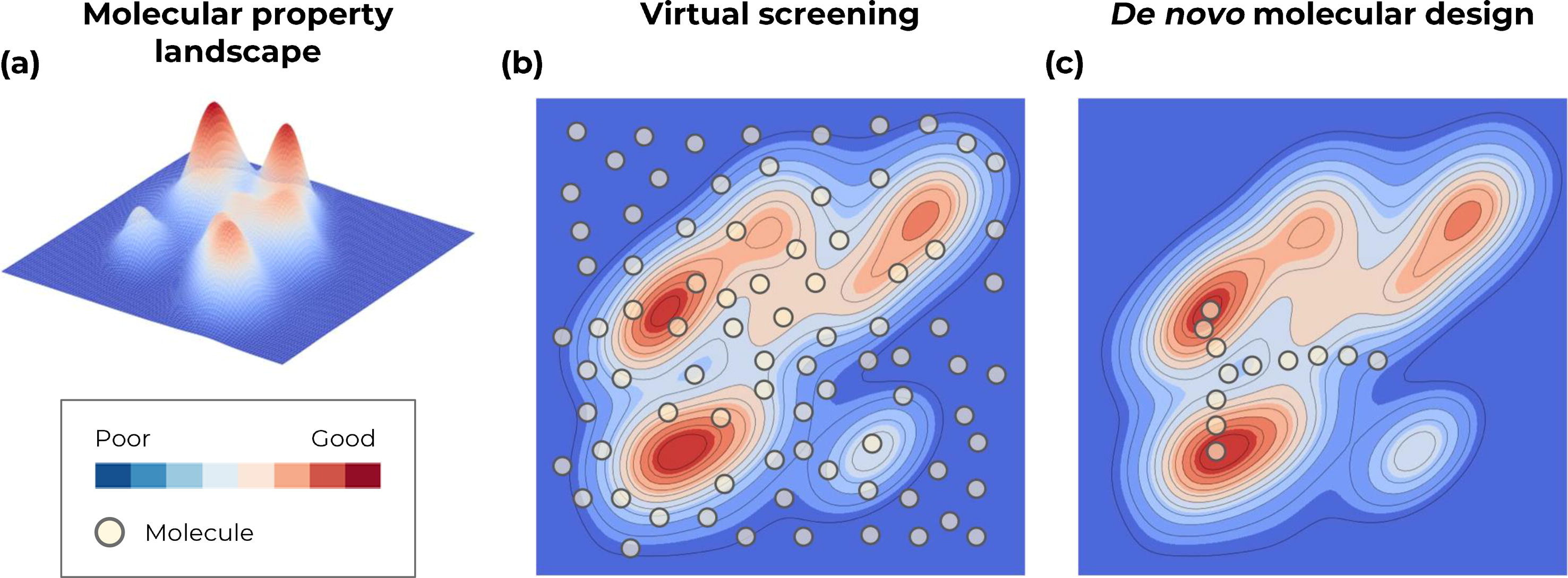
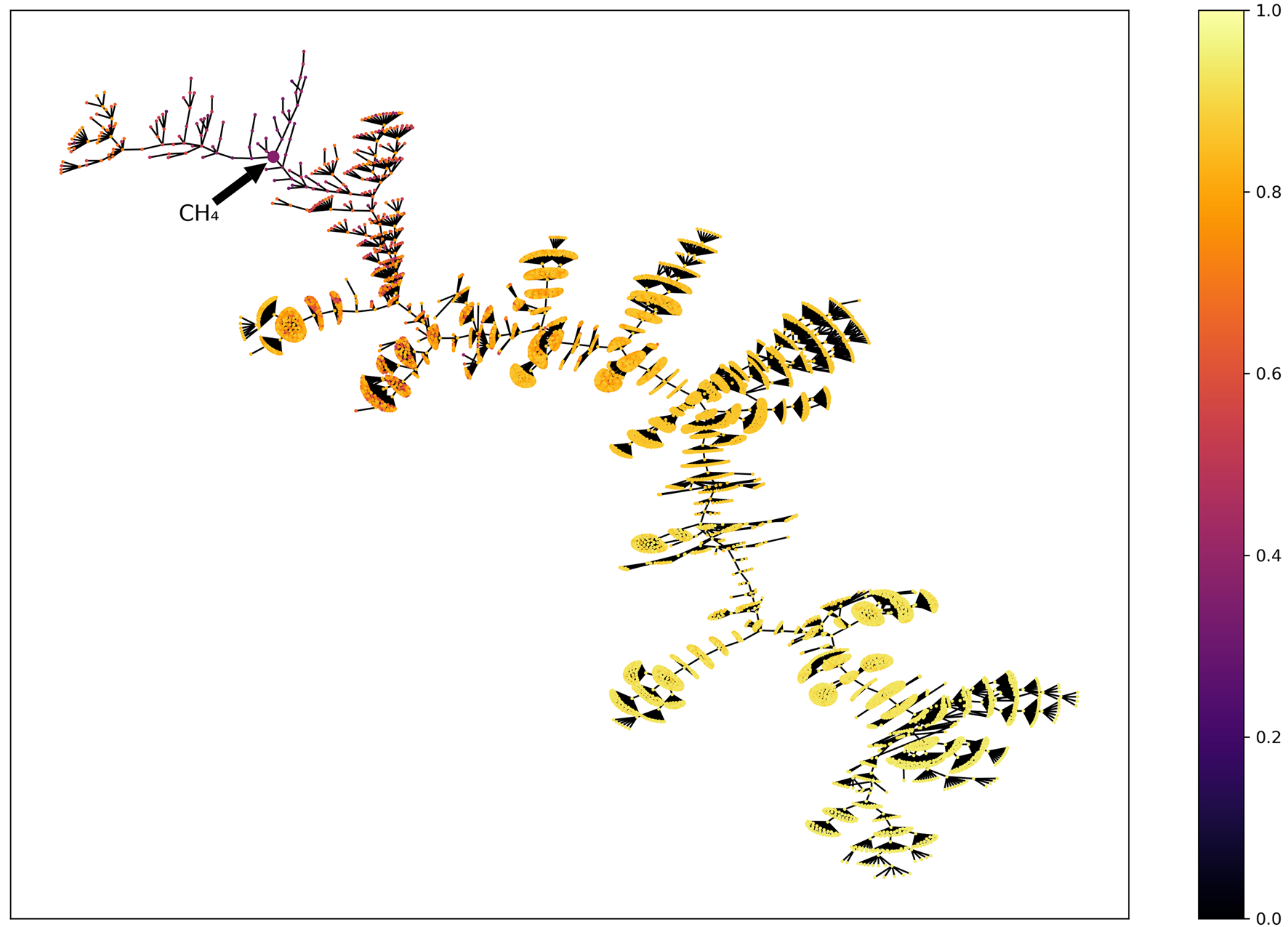
Main goal: Traverse the chemical space more effectively (better molecules in less evaluations)
- AI assisted de-novo design \(\rightarrow\) Process of automatically proposing novel chemical structures that optimally satisfy desired properties
De-novo molecular design
Generate compounds in a directed manner
- Reach optimal chemical solutions in fewer steps than VS
- Explore different acceptable regions of chemical space for a given objective (exploration vs. exploitation)
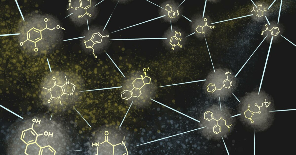
Recap - molecule encoding
- Molecules are 3D QM objects
- Encoding enables to capture certain information
- Trade-off: information loss vs. complexity

Generative and discriminative models
De-novo design is also referred to as generative chemistry
Discriminative models learn decision boundaries
Generative models model the probability distribution of each class
\(\rightarrow\) Can be instantiated to generate new examples (!)

Not the only way to obtain new compounds…
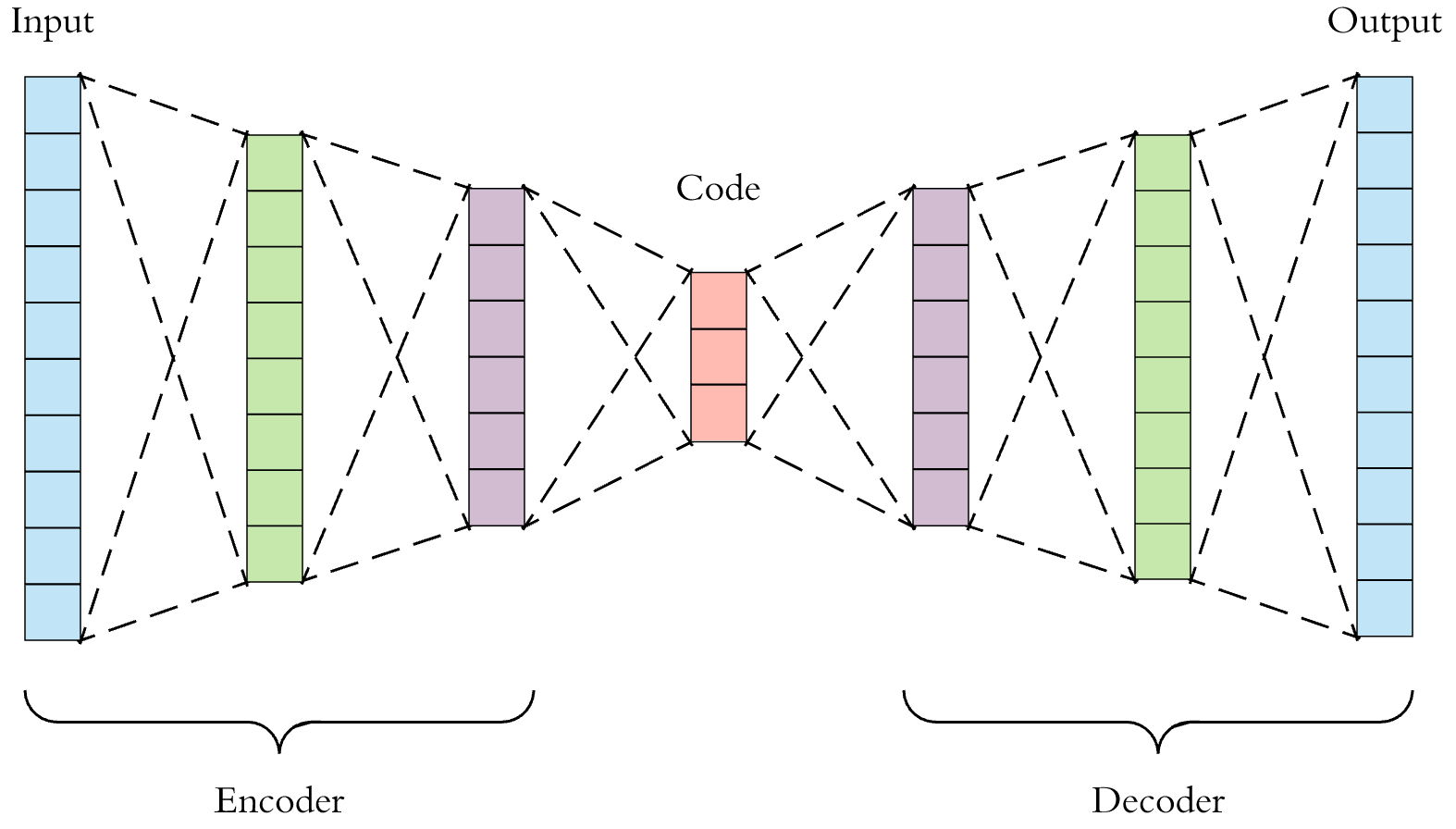
Autoencoder
AE: Hourglass-structured NN that encodes and decodes the input information, consisting on an encoder, \(f_\theta(x)\), decoder, \(g_\phi(z)\), and the latent space, \(z\)
Attempts to learn the identity function, i.e. \[ \text{VAE} = g_\phi \circ f_\theta \, \quad s.t. \quad \text{VAE}^*(x) = g_\phi(f_\theta(x)) = x \]
Autoencoder
AE can be seen as generative models
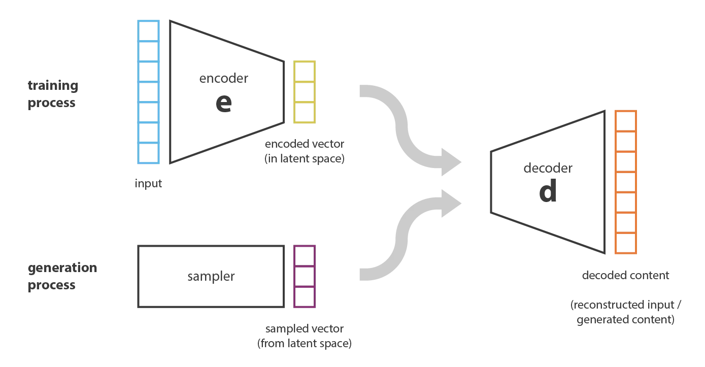
Latent space difficult to navigate
Variational Autoencoders
KL divergence as regularizer (closed form solution) \[ KL(q(z|x)|p(z)) = \sum_{i=1}^n (\sigma_{x,i})^2 + (\mu_{x,i})^2 - log(\sigma_{x,i})-1 \]
Adding noise, we sample from the latent space and decode it
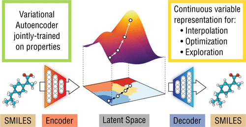
ChemVAE
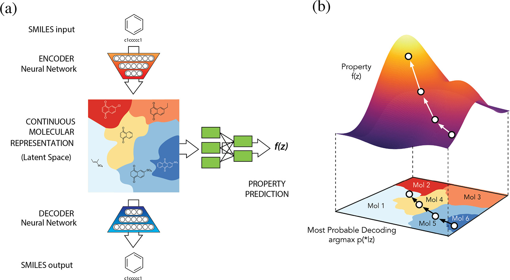
Fig: (a) ChemVAE architecture (b) Property optimization via BO
ChemVAE - Latent space
Local behavior + interpolation between compounds possible

ChemVAE - Latent space
Property prediction crucial for meaningful latent space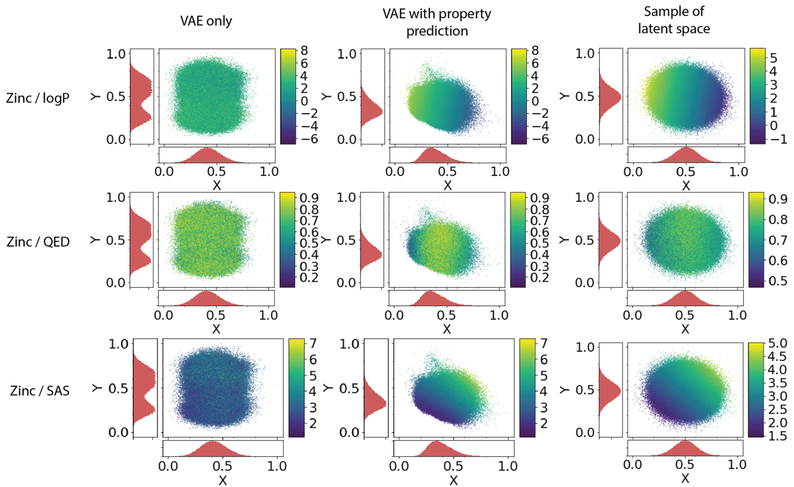
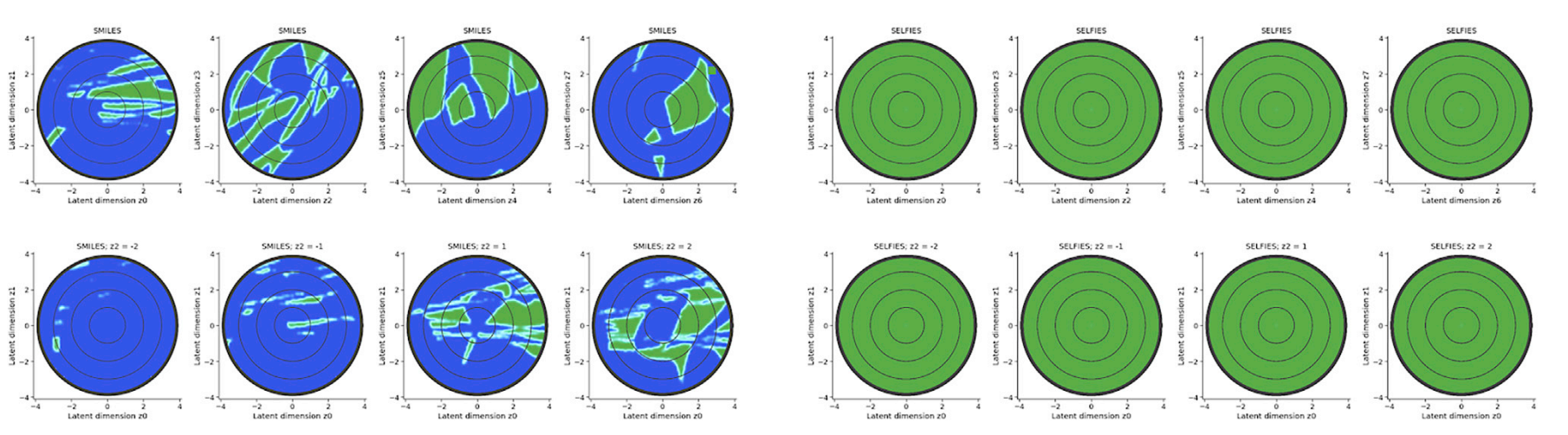
ChemVAE - Comments
ChemVAE - Hands on!
generative_models/ variational_autoencoder/ VAE.ipynb
Only a brief introduction though… Check the original repo for extended functionality
Other models
VAE-based: Recent interest in using reinforcement learning
- PaccMannRL: RL-based approach using 2 VAEs
- Used for SARS-CoV-2 drug discovery (paper)
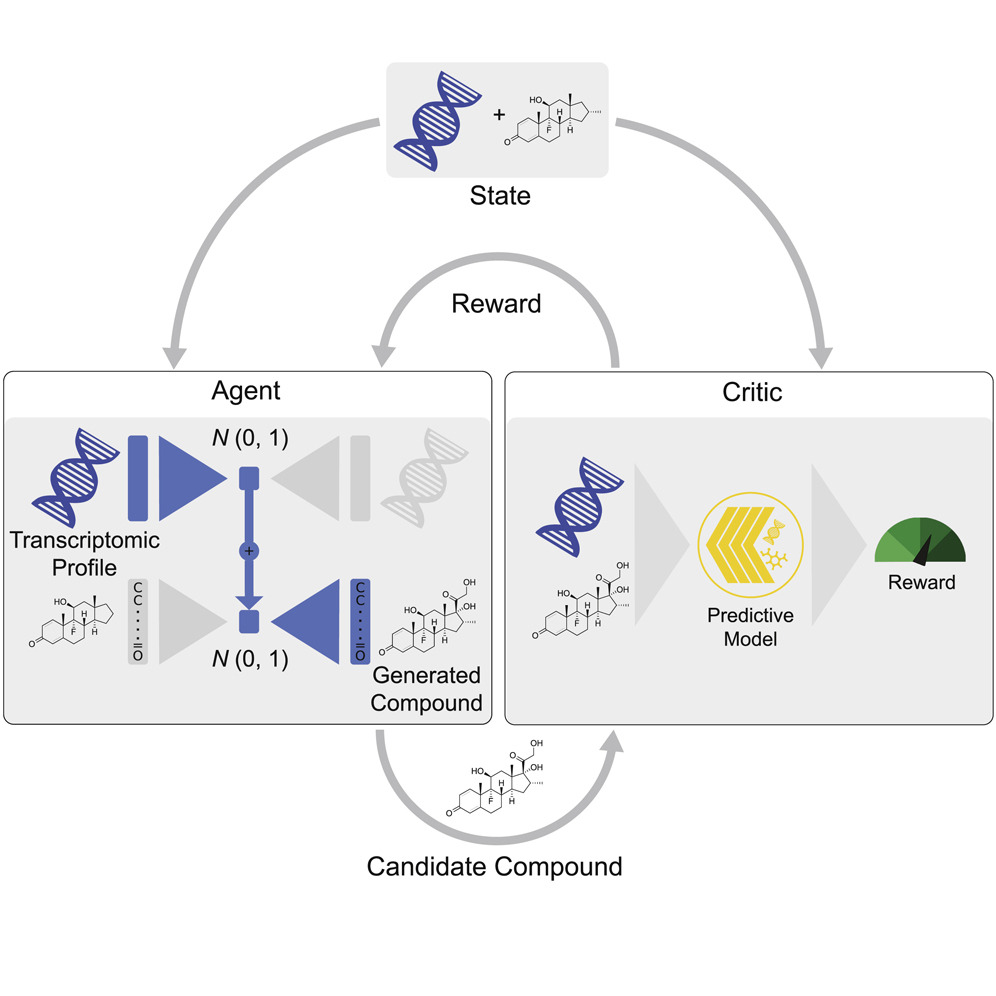
- Used for SARS-CoV-2 drug discovery (paper)
Diffusion models
EDM: Equivariant diffusion model for 3D molecule generation
- Use a diffusion process instead of a VAE
- \(E(3)\) symmetries: rotation, traslation and reflections
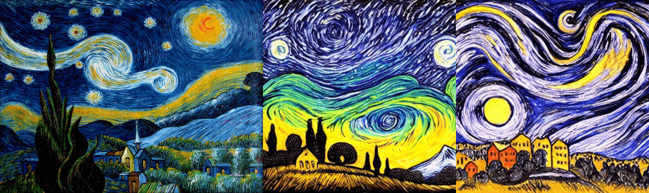
The same principle behind Stable Diffusion
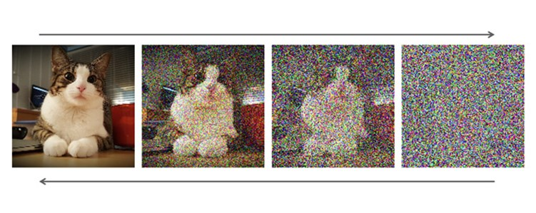
Diffusion models - diffusion process
Diffusion model learns denoising processes (opposite of a diffusion process)
\(\rightarrow\) progressively add Gaussian noise (\(z_t\)) to signal (\(x\)) \[ q(z_t|x) = \mathcal{N}(z_t|\alpha_tx_t, \sigma_t^2I) \] with \(\alpha_0 \approx 1\) and \(\alpha_T \approx 0\) and \(\sigma_t\) the added noise level
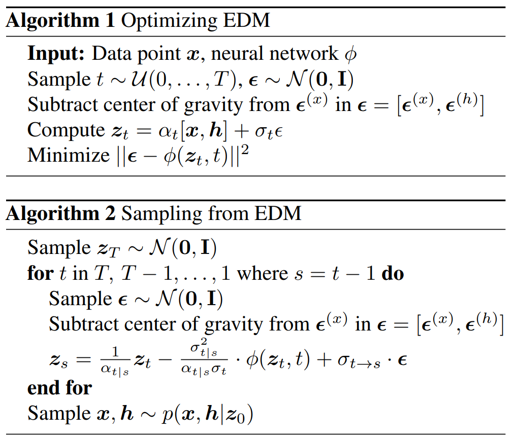
EDM - Overview
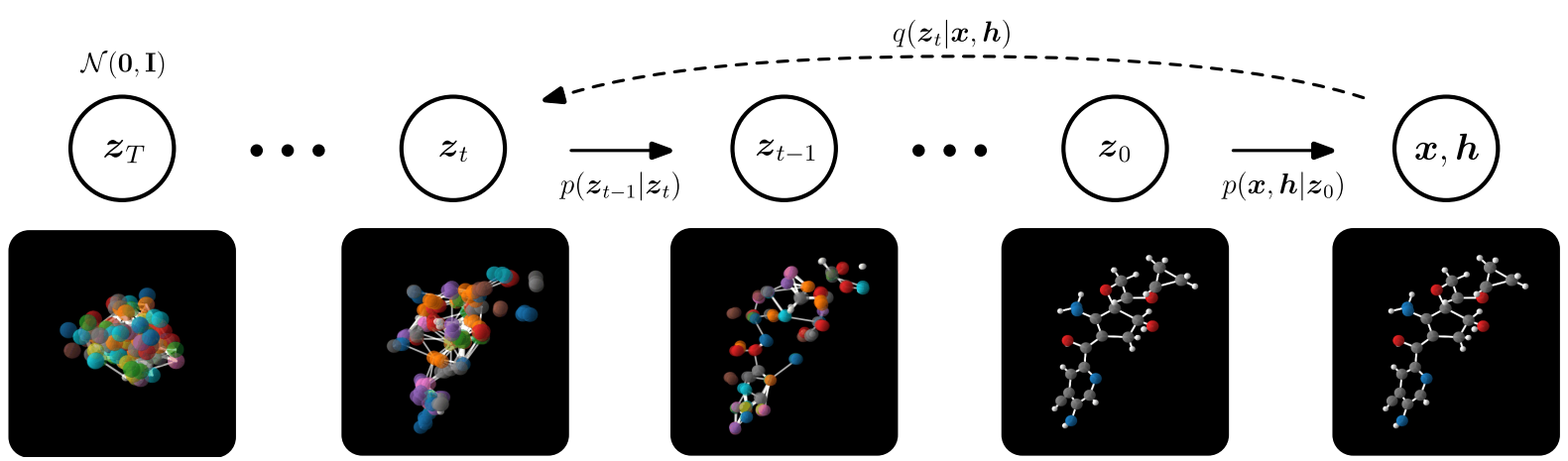
Similar to VAE approach, but now only decoding and latent space as pure noise
EDM - Computations
EDM - Conditional generation
EDM performs property optimization with a simple extension of \(\phi\) into \(\phi(z_t, [t, c])\), with \(c\) a property of interest

- Molecules with increasing polarizability (\(\alpha\)), given above
EDM - Hands on!
generative_models/ diffusion/DIFFUSION.ipynb
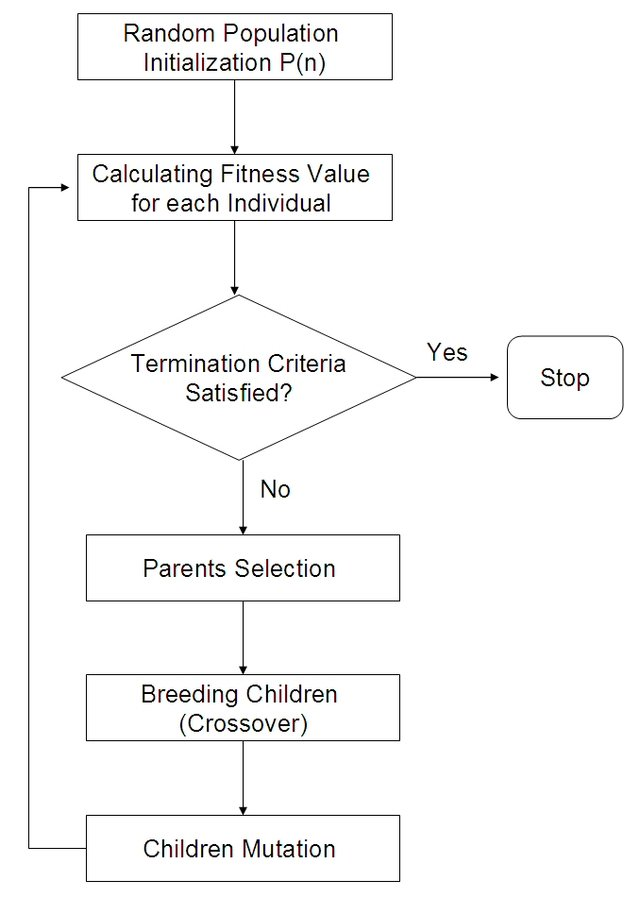
Evolutionary algorithms
Key idea:
Population of individuals (states) in which the fittest (highest valued state) produce offspring (successor states) that populate the next generation in a process of recombination and mutation.
Evolutionary algorithms
Many different evolutionary algorithms, they mostly vary on their setup regarding common criteria:
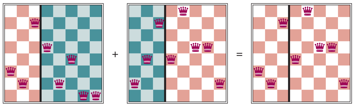
- Recombination procedure
- E.g. \(\rho = 2\), select random crossover point to recombine two parents into two children
Evolutionary algorithms
Example: (a) Rank population by fitness levels (b), resulting in pairs (c) from mating and producing offspring (d) which are subject to mutations (e)

Evolutionary algorithms
Child gets the first three digits from the \(1^{st}\) parent (327) and the remaining five from the \(2^{nd}\) parent (48552)
(no mutation here)
Evolutionary algorithms
Schema: Structure in which some positions are left unspecified
- Instances: Strings that match the schema
- Example: 327\(^{*****}\) (all instances beggining with 3, 2, and 7)
- Useful to maintain an interesting piece in evolutionary process

EvoMol
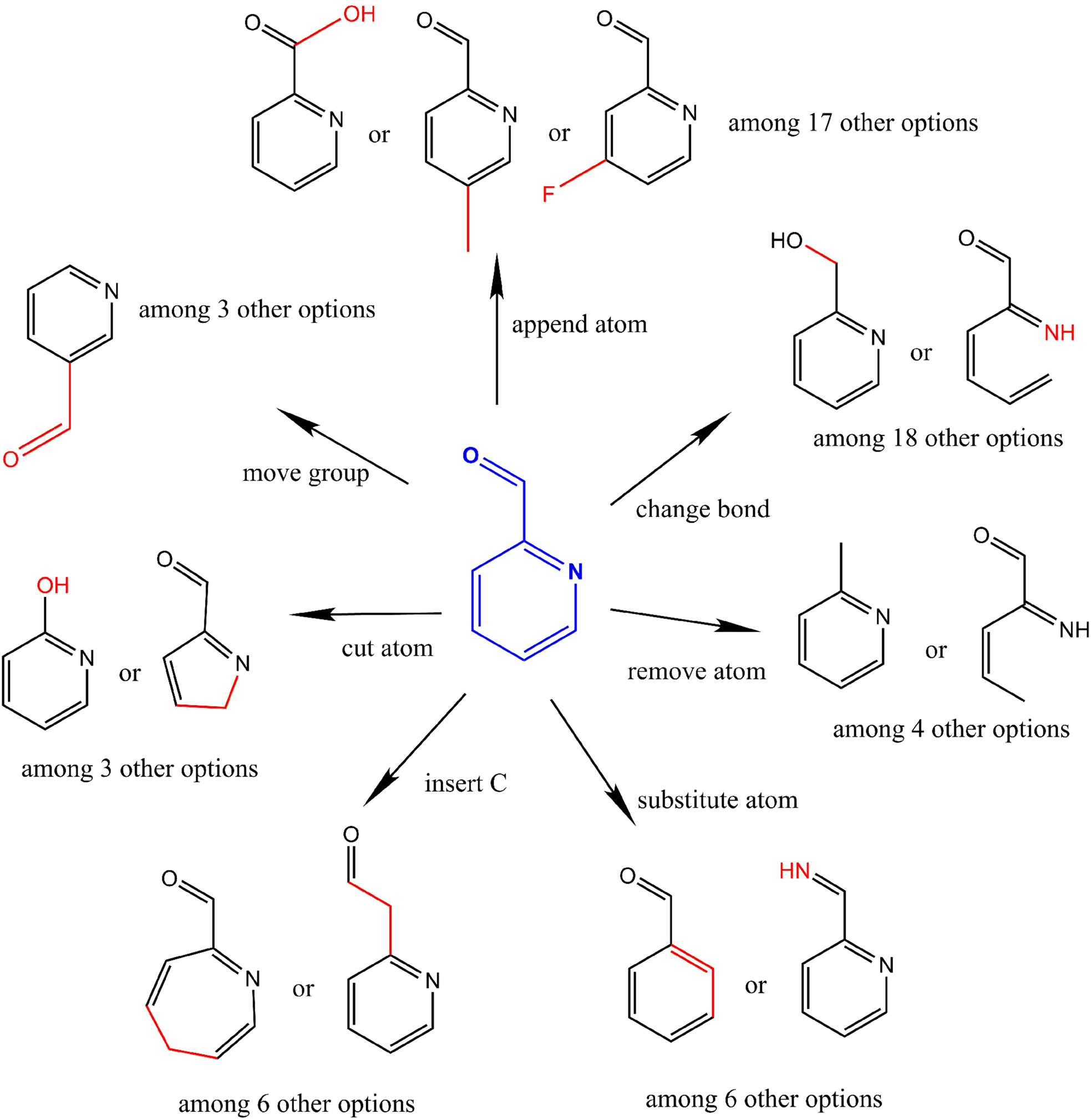
EvoMol - Impletation

EvoMol - Hands on!
generative_models/ evolutionary_algorithm/GENETIC.ipynb