Can Small Data Manipulations Compromise ML-Based Decisions?
CUNEF University
Collaborating with Doctors
- A few years ago, I collaborated with (medical) doctors studying uterine fibroids (myomas).

Comparing Medical Procedures
Doctors compared two minimally invasive treatments for myomas to determine which:
- Is more effective at reducing fibroid size.
- Is less invasive for patients, measured by shorter hospital stays, lower blood loss, etc.
Procedures Compared:
- Radiofrequency Ablation (RFA)
- Uterine Artery Embolization (UAE)
Doctors’ Initial Expectations
Doctors initially expected RFA to outperform the alternative treatment:
- More effective at reducing myoma size.
- Less invasive, resulting in shorter hospital stays and quicker recovery.
Biased toward RFA!
Disappointing Results…
Statistical analysis revealed no significant differences between RFA and the alternative treatment regarding length of hospital stay.
Data did not support the doctors’ initial preference for RFA!
A “Statistical Adjustment” Suggestion
One doctor asked:
“Can we perform a statistical adjustment to make RFA look better?”
And I replied
“What do you mean by ‘statistical adjustment’?”
Doctor:
“Look, if we remove this patient with an unusually large myoma from the RFA group, the results become significant!”
Wait… Can We Do That?
- This is not how stats work!
- But this inspired a deeper question:
How can one systematically select a minimal subset of data points to manipulate in order to alter a statistical/ML-based conclusion?
Background
Adversarial Machine Learning (AML), studies
How data manipulations influence ML-based inferences, predictions, and decisions.
How to design robust ML methods that are resistant to such manipulations.
We wil give an overview of AML attacks and defenses in the context of Bayesian Machine Learning.
The Problem
Honest Bayesian (Defender) observes training data \mathcal{D}_n = \{(X_i, y_i)\}_{i=1}^n.
Model: y_i \mid X_i, \theta \sim p(\cdot \mid X_i, \theta) with prior \theta \sim \pi(\theta).
Goal: update beliefs about the unknown parameter \theta \in \mathbb{R}^d based on observed data.
The Bayesian Update
Posterior = prior x fit to the observed pairs: p(\theta \mid \mathcal{D}_n) \propto \underbrace{p(\theta)}_{\text{prior}} \times \underbrace{\prod_{i=1}^n p(y_i \mid X_i, \theta)}_{\text{likelihood of the observed pairs}}
- Score how well each \theta explains all pairs (X_i,y_i), reweight the prior, and then normalize.
- Typically approximated with MCMC or variational inference.
Posterior Predictive Distribution
- For a new covariate vector x_{\text{new}}, we average over all plausible parameter values.
p(y_{\text{new}} \mid x_{\text{new}}, \mathcal{D}_n) = \int p(y_{\text{new}} \mid x_{\text{new}}, \theta)\,p(\theta \mid \mathcal{D}_n)\,d\theta
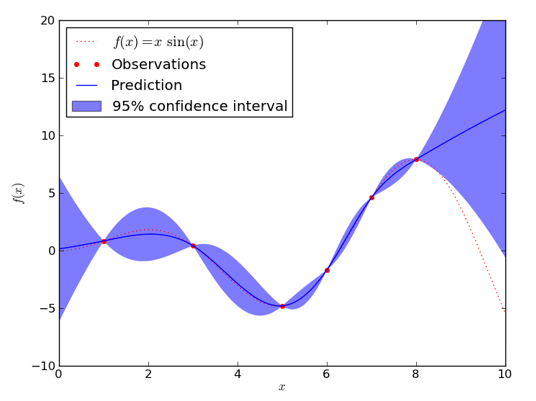
- The predictive distribution not only gives a point prediction but also quantifies uncertainty about future outcomes.
UQ Example
The Bayesian Approach to Decision-Making
A decision means choosing an action a \in \mathcal{A}.
A utility u(a,s) tells us how desirable the consequence is if we take action a and state s happens.
In our setting, s could be an unknown parameter \theta or a future outcome Y_{\text{new}}.
The Bayesian Approach to Decision-Making
- We model our uncertainty about the state s with a probability distribution p(s \mid \mathcal{D}_n), which could be the posterior or the predictive distribution.
The Bayesian Approach to Decision-Making
- In utility theory, a rational/coherent agent is one whose choices satisfy standard rationality axioms. A rational agent chooses the action that maximizes expected utility.
a^* = \arg\max_{a \in \mathcal{A}} \int u(a,s) p(s | \mathcal{D}_n) ds
- In words: average the utility of each action over your posterior uncertainty, then pick the best one.
Why This Matters
In Bayesian ML, even small data manipulations can propagate through the pipeline and ultimately alter the decision induced by the model.
An attack may target posterior inference, posterior prediction, or directly the final decision rule.
In the rest of the talk, I focus on attacks on inference and prediction.
Example: Mexico Microcredit Data
Randomized controlled trial on microcredit (16,560 businesses) conducted in Mexico City (Angelucci et al., 2015).
Treatment assignment: x_i = \begin{cases} 1 & \text{microcredit} \\ 0 & \text{control} \end{cases}
Objective: Assess impact on business profit y_i.
Example: Mexico Microcredit Data
Model used, parameters are \theta = \lbrace \beta_0, \beta_1, \sigma \rbrace: p(y_i \mid X_i, \theta) = \mathcal{N}(\beta_0 + \beta_1 x_i, \sigma^2)
Priors: p(\theta) \beta_0,\,\beta_1,\, \log(\sigma) \sim t(3,\,0,\,1000)
Parameter \beta_1 represents the Average Treatment Effect (ATE).
It is the average change in profit caused by offering microcredit, so its sign and magnitude determine whether expanding the program looks beneficial or harmful.
Example: Mexico Microcredit Data
We observe data \mathcal{D}_n = \{(X_i, y_i)\}_{i=1}^n.
n = 16,560
We approximate posterior p(\beta_0, \beta_1, \sigma | \mathcal{D}_n).
Posterior for the ATE
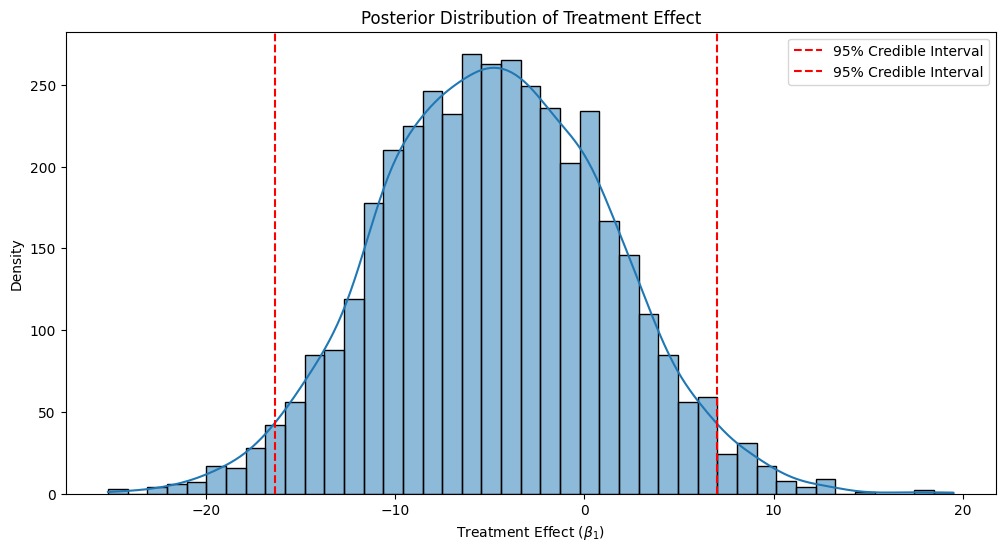
- Posterior mean of ATE (\beta_1): -4.71 (negative impact).
- Potential policy implication: Do not expand microcredit.
From Posterior to Decision
- Consider two actions: a \in \{\text{expand}, \text{do not expand}\}.
- Suppose the policymaker utility is (c is expansion cost). u(\text{expand}, \beta_1) = \beta_1 - c, ~~ u(\text{do not expand}, \beta_1) = 0
From Posterior to Decision
Then expected utility for expanding is: \mathbb{E}[u(\text{expand}, \beta_1) \mid \mathcal{D}_n] = \mathbb{E}[\beta_1 \mid \mathcal{D}_n] - c = -4.71 - c,
For not expanding: \mathbb{E}[u(\text{do not expand}, \beta_1) \mid \mathcal{D}_n] = 0
Since c > 0, we have -4.71 - c < 0, so the Bayes action is: do not expand microcredit.
Attacking Posterior Inferences
Attacker manipulates data by deleting or replicating points.
Represented by integer vector w \in \mathbb{Z}_{\geq 0}^n:
- w_i = 0: remove data point i
- w_i > 1: replicate data point i
- w_i = 1: no change
The Attacker
Resulting posterior: \pi_w(\theta \mid \mathcal{D}_n) = \frac{1}{Z(w)} \left(\prod_{i=1}^n p(y_i \mid X_i, \theta)^{w_i}\right)\pi(\theta)
Goal: alter statistical conclusions by manipulating just a few data points.
The Attack
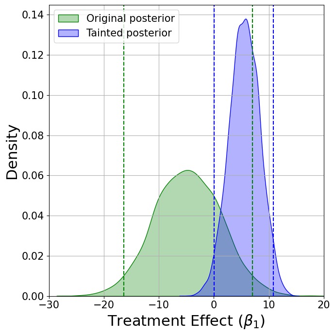
Just removing a strategically chosen 0.12 \% (B=20) of the data points…
The Attack
- Now the optimal decision is to actually expand the microcredit program!!
How do we find the points to manipulate?
Goal: Find minimal data manipulations w \in \mathbb{Z}_{\geq 0}^n such that the resulting posterior \pi_w(\theta \mid \mathcal{D}_n) is as close as possible to a target distribution \pi_A(\theta).
Formalizing the Adversary’s Problem
Minimize forward KL divergence: \min_w \quad \text{KL}(\pi_A(\theta) \parallel \pi_w(\theta \mid \mathcal{D}_n))
Subject to constraints: w \in \mathbb{Z}_{\geq 0}^n, \quad \|w - \mathbf{1}\|_1 \leq B, \quad \|w\|_\infty \leq L
But…
- Exact posterior often intractable (unknown normalization constant).
- There is no closed-form expression for the objective function.
- If curious see here.
Attacks can also target predictions!
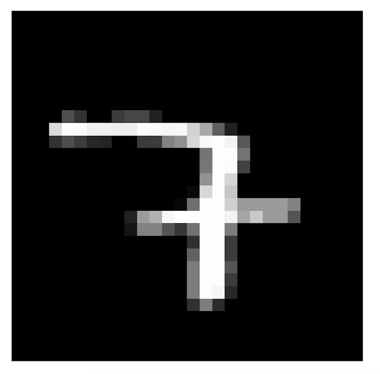
Imagine a BNN trained on MNIST to classify digits.
Data: \mathcal{D}_n = \{(x_i, y_i)\}_{i=1}^n, where x_i is an image and y_i \in \{0,\dots,9\} is its label.
Representation (model and prior): put a prior on the network weights W, and let the network define p(y \mid x, W).
BNN for MNIST Classification
- Training: update this prior into a posterior p(W \mid \mathcal{D}_n) \propto p(W)\prod_{i=1}^n p(y_i \mid x_i, W), typically approximately with variational inference or stochastic-gradient MCMC.
BNN for MNIST Classification
Prediction: average the network outputs over posterior draws of the weights p(y_{\text{new}} \mid x_{\text{new}}, \mathcal{D}_n)= \\ \int p(y_{\text{new}} \mid x_{\text{new}}, W)\,p(W \mid \mathcal{D}_n)\,dW.
Infinite ensemble of networks, each weighted by how well it explains the training data.
BNN for MNIST Classification
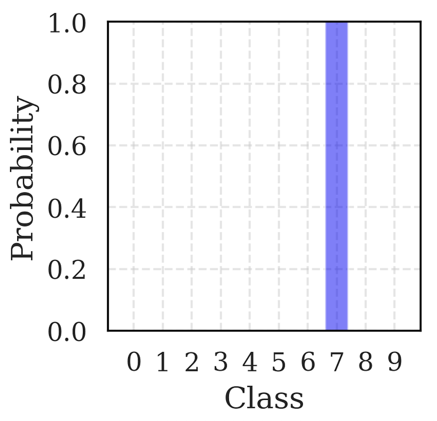
Formalizing the Attack on BNN Predictions
Start from a clean image x and its BNN predictive distribution p(y \mid x,\mathcal{D}_n).
Unlike before, the attacker perturbs the test image itself, while leaving the training data untouched.
Formalizing the Attack on BNN Predictions
The attacker can only make a small change to the pixels: \mathcal{X}(x)=\{x' : \|x'-x\|\leq \epsilon\}.
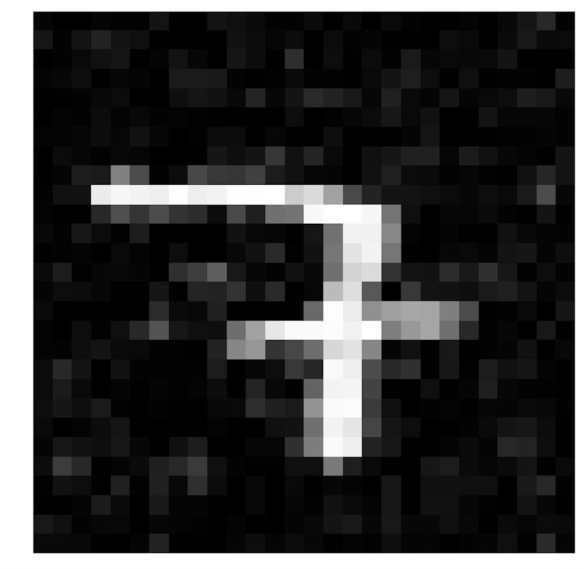
Concrete example: the clean image is a 7, but the attacker wants the BNN to believe it is a 3. Make p(Y=3 \mid x',\mathcal{D}_n) as large as possible.
Formalizing the Attack on BNN Predictions
- The attacker looks for a perturbed image x' that still looks similar to the original one, but maximizes the probability of class 3.
x^*_{\text{adv}} = \arg\max_{x' \in \mathcal{X}(x)} p(Y=3 \mid x',\mathcal{D}_n)
- In words: among all small perturbations, find the one that makes the BNN say “3” as confidently as possible.
Solving the Attack Problem
Approximate the predictive probability with posterior samples W^{(1)},\dots,W^{(M)}: p(Y=3 \mid x',\mathcal{D}_n) \approx \frac{1}{M}\sum_{m=1}^M p(Y=3 \mid x', W^{(m)}).
We estimate \nabla_{x'} p(Y=3 \mid x',\mathcal{D}_n) by backpropagating through the network.
Then we update x' with projected gradient ascent steps, projecting back onto \mathcal{X}(x) after each step.
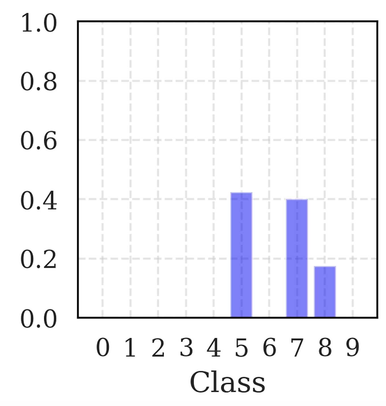
Attack on BNN Predictions
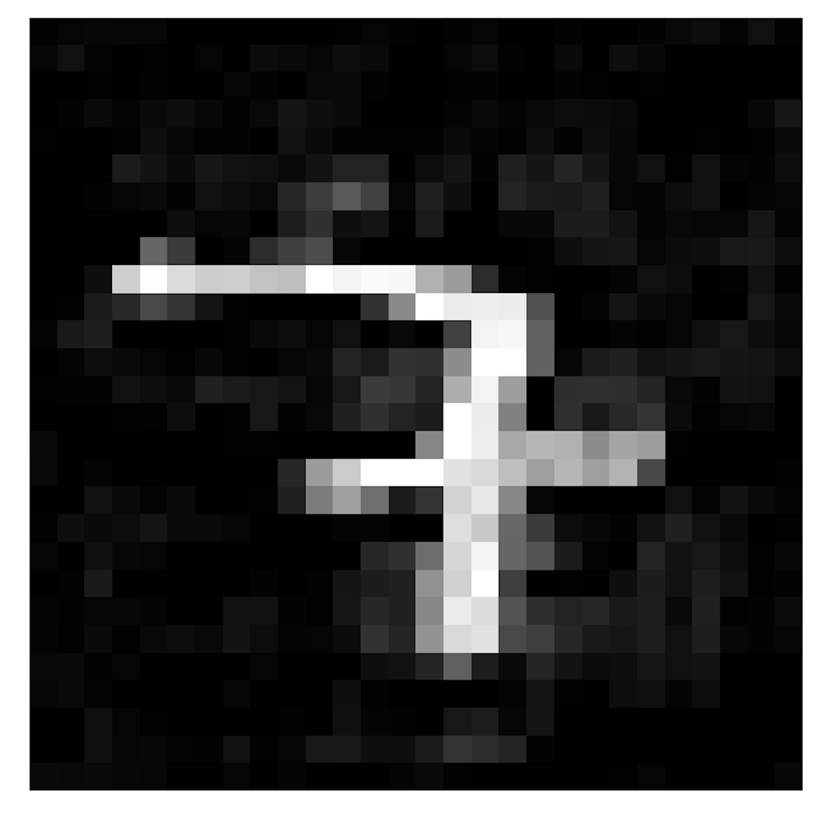
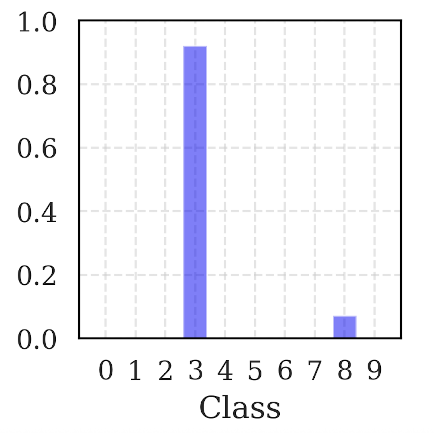
Attacks on uncertainty quantification
The attacker can also target the BNN’s uncertainty estimates.
Make them overconfident in wrong predictions, or underconfident in correct ones.
Attack on BNN Predictions
What’s going on?
It seems that NNs (on clean data) learn superficial patterns that are not robust to small perturbations
i.e. they are not learning the true underlying concepts, but rather some shortcuts that work well on clean data but fail under adversarial conditions.
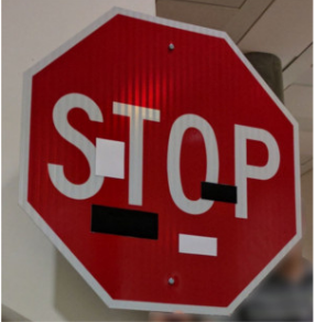
This is very serious for safety-critical applications like autonomous driving, medical diagnosis, etc.
Autonomous Driving Example
Defending Against Attacks
- Suppose we knew exactly how a clean input x is turned into an attacked input x'.
- Then two natural defenses are:
- Purification: try to invert the attack and recover the clean input.
- Adversarial training: train the network directly on attacked images.
- Both ideas depend on knowing, at least approximately, how the attacker behaves.
But Usually We Do Not
In practice, we do not know which attack will be used, how strong it will be, or how often it will appear.
Bayesian view: model all the known unknowns.
Not only model the data y | x, \theta, also model the attacker through a probabilistic adversarial channel p(x' \mid x,\theta), which represents a distribution over plausible perturbations.
But Usually We Do Not
Then purification and training can average over likely attacks, instead of assuming one fixed perturbation.
Caveat, modelling humans, is hard (performative effects, infinite regressions, etc.)
Game Theory, Adversarial Risk Analysis.
Conclusions
Small, plausible perturbations can change Bayesian posteriors, predictions, and therefore decisions.
This is especially serious in safety-critical settings.
So defenses should model the attacker probabilistically and train against a distribution of attacks.
Arms race!
Thank You!
Questions are welcome!
📧 roi.naveiro@cunef.edu
🌐 https://github.com/roinaveiro